Kategorie: Nouvelle

Diese Seite presentiert ein Anwendungsbeispiel des Programms Siam.

Schritt 1: Öffnung eines neues Fensters.

Es wird ein leeres Fenster erzeugt (Bild 1).

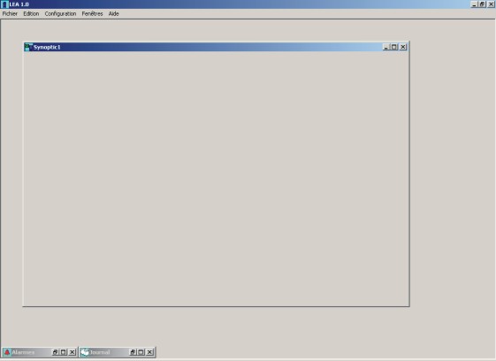
Bild 1 Ein leeres ‚Synoptic‘ Fenster

Schritt 2: Ein Bild importieren.

Das Bild kann zum Beispiel die zu automatisieren Installation enthalten (Bild 2).

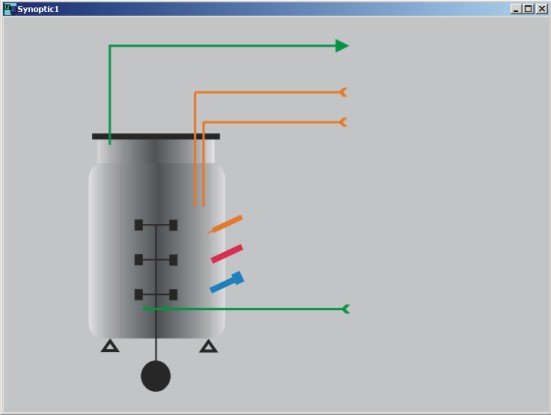
Bild 2 Ein ‚Synoptic‘-Fenster mit Bitmap-Bild

Schritt 3: Gewünschte visuelle Komponente im Fenster hinzufügen.

Der gewünschte Komponente wird aus der Toolbox selektiert .

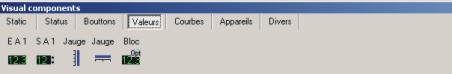
Bild 3 Toolbox für visuelle Komponent

Die gewählte visuelle Komponent wird durch klicken dort eingefügt, wo es der Benützer wünscht (Bild 4). Die einzelne Komponenten können bewegt oder gelöscht werden, solange das Programm im Konfigurationsmodus ist.

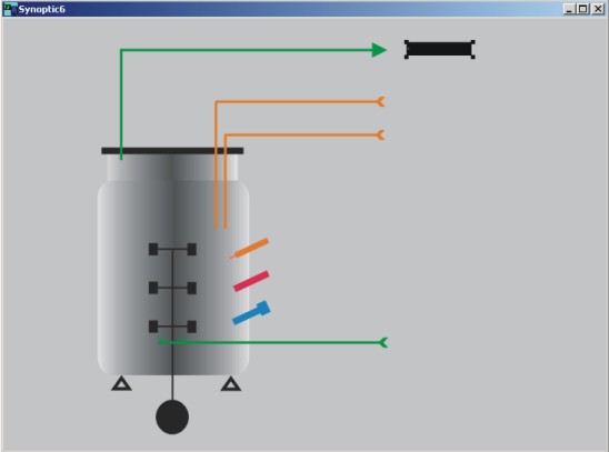
Bild 4 Eine visuelle Komponente einfügen

Schritt 4: Der Komponent mit einem Kanal verknüpfen

Um eine visuelle Komponente mit einem Kanal (Messung, Sollwert,…) eines Gerätes (Waage, A/D Wandler, etc…) zu verknüpfen, klickt man auf die Komponente mit der rechten Maustaste. Es wird ein Popupmenü angezeigt (Bild 5).

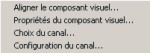
Bild 5 Popumenü für die Kanalwahl

Man klickt auf Kanalwahl. Es erscheint ein neues Fenster. Der Benutzer kann hier den Kanal, der er verknüpfen möchte, anwählen (Bild 6).

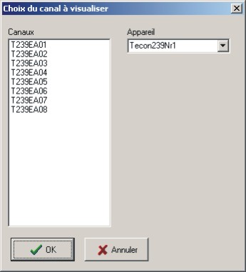
Bild 6 Auswahlliste der Kanäle, die der visuellen Komponente zugeordnet werden können

Schritt 5 : Verknüpfter Kanal konfigurieren

Der Kanal besitzt jetzt eine Grundkonfiguration. Um diese Konfiguration zu sehen oder zu ändern, klickt man mit der rechten Maustaste auf die Komponent. Es wird ein Popupmenü angezeigt (Bild 5). Man wählt jetzt die Option Kanalkonfiguration (Bild 7).

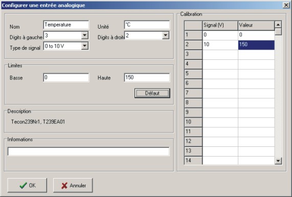
Bild 7 Konfiguration eines analogen Eingangs (hier z. B. Tecon 239)

Man kann zum Beispiel die Kanalname und die Kalibration ändern.

Schritt 6 und nachfolger: Die Erstellung und Verknüpfung weiterer visuelle Komponenten erfolgt genauso, d. h. mit dem Schritten 3-6.

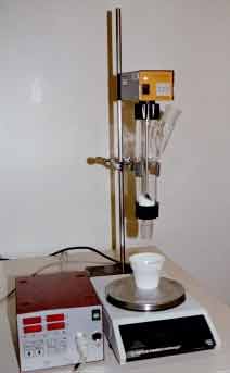
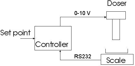
Das Gerät (hier das Interface Tecon 239) kann am PC angeschlossen werden und die Kommunikation gestartet werden.

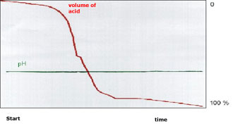
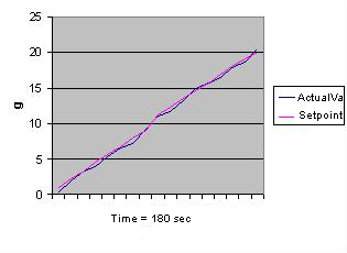
Bild 8 zeigt ein Beipiel für ein so erstelltes Fenster. Auch Fenster mit Trendkurven können auf diese Weise einfach erstellt werden.

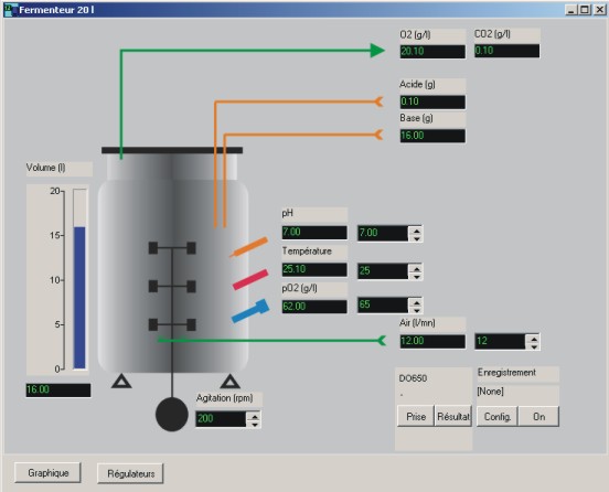
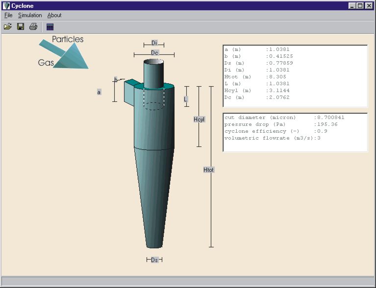
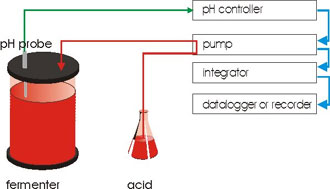
Bild 8 Beispiel: Automatisierung eines Fermenters

Diese Konfiguration kann gespeichert und später modifiziert oder erweitert werden. Für spätere Anpassungen bietet die Software Siam, z. B. mit Waagen, zusätlichen Sensoren oder Reglern, eine sehr hohe Flexibilität.

This example shows how to use the software Cyclone to calculate a cyclone. With a few known parameters, the software will calculate the unkown parameters, like the cyclone dimension and the efficiency for different particles size.

Known parameters air flow rate: 3 m3/s

pressure: 1 bar

gas is air at room temperature: 293 °K

solid density is : 1500 kg /m3

solid distribution is:

particule diameter (micron)	inferior cumulated frequency
8	0.07
12	0.13
24	0.3
32	0.5
48	0.86
64	0.94
78	0.99
96	1

overall efficiency should be: 0.92

Parameters to calculate

cyclone dimension

efficiency depending on the particule size

pressure drop in the cyclone

Calculation

Step 5. Choose a model in the list. Here the simualtion has been made with the Lorenz model. Eventually it is possible to enter a particule diameter distribution to calculate the efficiency for every particule size class (not possible with the Barth model).

Then press the simulation button.

The software give you in this case the cyclone dimension, the cut diameter and the pressure drop.

Conclusion. With the software Cyclone, you can easily calculate the dimension of a cyclone, without to enter one formula. The software calculations are very quick wich allow you to compare different cyclone parameters in a short time.

In many processes it is necessary to know the amount of a component which was added. The Lambda Integrator now integrated in the Preciflow pump, can monitor the amount of liquid added. 1. Presentation of the installation (figure 1) During a fermentation, maintainance of the pH value is necessary, wich is achieved by addition of acid. A pH controller measures the pH and gives a signal to the pump if addition of acid is necessary. The input of the Lambda integrator is coupled with the pump and the output of the integrator gives an electric signal that is proportional to the amount of liquid that has been added. In summary by use a voltmeter, a recorder or a datalogger, it is possible to visualize on line the amount of acid added.

figure 1

2. Result (figure 2)

Keeping the pH value constant during a whole fermentation. The green line visualises the pH value in the fermenter and the red curves shows the amount of acid added. At the beginning the addition of the acid is slow. With the time the biomass grows wich leads to a increase of the addition of acid. At the end of the biomass growth decrease and so does the amount of acid added.

The Integrator can also be used to monitor enzyme activity ( amidase,…).

We present here a set of devices wich connected together permit to add a defined amount of powder in a flask, fully automatically. Material and methods A PID controller ist connected to a balance trough a serial RS232 interface (fig. 1 and 2). The doser, wich contains the powder ist controlled by a 0-10 V signal. With 0 V the doser ist stopped, with 10 V it has maximal speed.
					figure 1 The devices
		figure 2. The connection between the devices
The user enter the amount of powder he want and the duration of the dosing. He press then the start button. The controller calculate at each time the amount of powder which should be added (set point). It compare this value with the weight measured at the scale, and control the speed of the doser. This configuration has been used to add 3 time 5 g, and 3 time 20 g of NaCl powder. The controller parameter P=2 (proportional) and D = 0 (differential) have been used for this experiment. Results The results are reported in the table below. The figure 3 shows set point profile calculated from the controller (red) and the added powder (blue) in fonction time. On this curve you can see how the controller adjust the added amount to the calculated setpoint, wich follows a line.
Set point (g) 5 5 5 20 20 20 Dosing time (min) 2 2 2 3 3 3 Powder amount measured (g) 4.8 5.2 5.3 20.4 20.1 20.0
figure 3. Amount of powder added in function of time Conclusion The addition of powder with the doser has a good reproductibility , and a good precision (better then 0.5 g) The same construction can be made for liquid by replacing the doser with a peristaltic pump. A new controller is in preparation. It will accept set point with 0.1 g precision.